Normalized Cut

08 Jul 2022 in Paper

참고
[1] https://people.eecs.berkeley.edu/~malik/papers/SM-ncut.pdf

---

코드
https://github.com/tinnunculus/Ncut/blob/master/Ncut.ipynb

---

• Introduction
• Conventional Cutting algorithm
• Normalized Cut
• Computing the Optimal Partition
• Grouping Algorithm
• Example: Brightness Images
• Review

Introduction

• 이 논문은 2000년도에 출간된 논문으로 Spectral Graph Theory를 기반으로 새로운 Graph Partitioning 기법을 제시한다.
• 기존에 있던 Graph Cutting 알고리즘에 문제를 해결하는 새로운 Graph Cutting 기법인 Normalized Cut 알고리즘을 만들었다.
• 새로운 Normalized Cut 알고리즘의 NP 문제를 generalized eigenvalue problem으로 접근해 효율적으로 해결하였다.

Conventional Cutting algorithm

• 그래프 \(G = (\mathbf{V}, \mathbf{E})\) 를 두개의 disjoint sets \(\mathbf{A}, \mathbf{B}, \mathbf{A} \cup \mathbf{B} = \mathbf{V}, \mathbf{A} \cap \mathbf{B} = \emptyset\) 으로 나누는 문제를 Graph Cut이라고 한다.
• 그래프는 노드의 집합 \(\mathbf{V}\) 와 두 노드간의 similarity를 나타내는 집합 \(\mathbf{E}\) 로 구성되어있다.
• 두개의 sets \(\mathbf{A}, \mathbf{B}\) 의 association의 척도를 나타내는 함수를 \(asso(\mathbf{A}, \mathbf{B})\) 라고 한다.

\[assoc(\mathbf{A}, \mathbf{B}) = \displaystyle\sum_{u \in \mathbf{A}, v \in \mathbf{B}} w(u, v)\]

• Optimal Graph Partitioning은 \(assoc(\mathbf{A}, \mathbf{B})\) 의 값을 최소화 시키는 \(\mathbf{A}, \mathbf{B}\) 을 찾는 것이다. 즉 가장 dissociation한 두개의 disjoint set \(\mathbf{A}, \mathbf{B}\) 을 구하는 문제이다.
• 전체 set \(\mathbf{V}\) 을 두개의 sets \(\mathbf{A}, \mathbf{B}\)으로 나누어 지는 경우의 수는 exponential의 빅오를 가지기 때문에 매우 많은 계산량이 필요하지만, \(minimum asso\) 문제는 당시에도 well-studied problem 이었기 때문에 이 문제를 풀기 위한 효율적인 알고리즘이 존재했다.
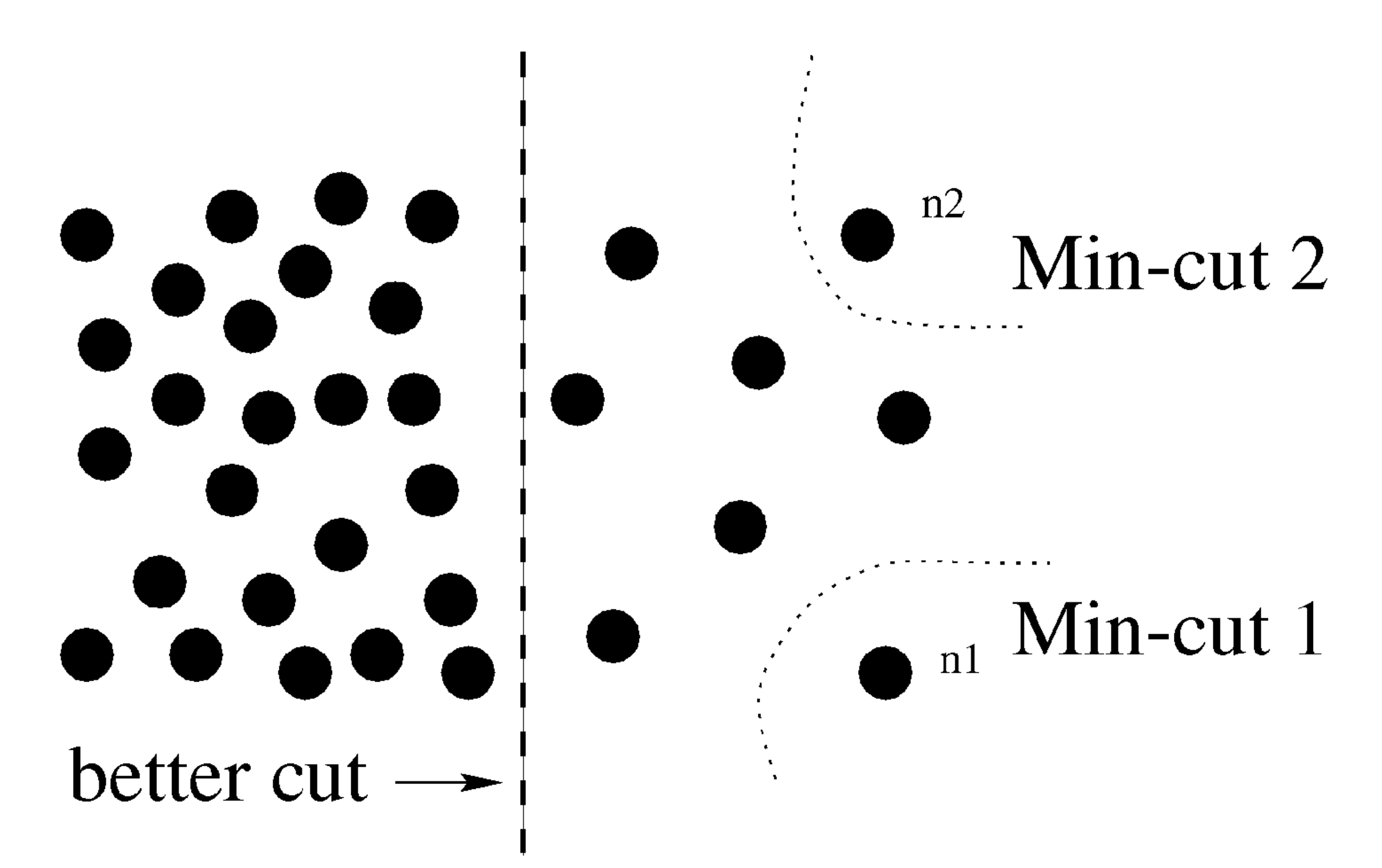
• 하지만 위의 식을 최소화 시키는 방향으로 Group을 Cutting하다 보면 Graph에서 혼자 고립된(similarity가 작은) 노드를 cutting하는 것을 선호한다. 즉, association 함수가 Normalized가 되지 않은 Summation으로 이뤄지기 때문에 Summation의 항의 수가 작은 방향으로 Cutting될 확률이 높기에 small set of node로 cutting되는 경향이 있다. 아래의 그림에서 노드 간의 거리가 가까우면 weight가 높은 그래프가 있다고 했을 때, 중앙의 선으로 partition하는게 이상적으로 보이지만, 실제로는 n1과 n2노드가 분리되는 방향으로 cutting이 진행된다.

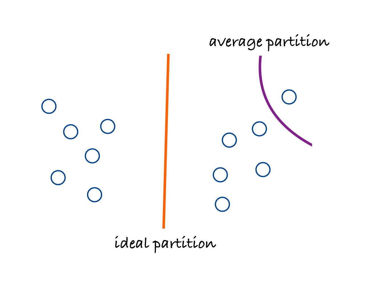
• 위의 문제는 단순히 Summation으로 assocation을 측정했기 때문이다. 그러면 Summation이 아닌 edge의 수로 나눠주는 normalized를 처리하면 문제가 해결될까..? 그렇지 않다. edge의 수로 normalized를 해도 똑같이 고립된(simmilarity가 작은) 노드를 컷팅하는 경향이 생길 것이다. 평균의 weight가 가장 작은 edge를 고르는 것이기 때문이다. 아래의 그림에서도 마찬가지로 중앙의 선이 아닌 가장 멀리 떨어진 하나의 노드를 나누는 식으로 cutting이 될 것이다.

Normalized Cut

• 본 논문에서는 새로운 Normalized Association 함수를 제시한다.
• 단순의 두개의 sets \(\mathbf{A}, \mathbf{B}\) 에 존재하는 similarity의 Summation이 아닌 연결된 전체 노드간의 비율로 계산을 한다.

\[\begin{aligned} Nassoc(\mathbf{A}, \mathbf{B}) = \frac{assoc(\mathbf{A}, \mathbf{B})}{assoc(\mathbf{A}, \mathbf{V})} + \frac{assoc(\mathbf{A}, \mathbf{B})}{assoc(\mathbf{B}, \mathbf{V})} \end{aligned}\]

• 새로운 Assocation 함수를 이용하면 기존 알고리즘에서 문제가 되었던 고립된 노드를 걷어내는 식으로 Cutting이 되는 경향을 해결할 수 있다.
• 한쪽 set의 노드 수가 다른 set보다 극히 작응면 \(Nassoc\) 함수의 한쪽 항은 0, 다른 항은 1에 가까워지기 때문이다.
• 또한

\[\begin{aligned} Nassoc(\mathbf{A}, \mathbf{B}) &= \frac{assoc(\mathbf{A}, \mathbf{B})}{assoc(\mathbf{A}, \mathbf{V})} + \frac{assoc(\mathbf{A}, \mathbf{B})}{assoc(\mathbf{B}, \mathbf{V})} \\[1em] &= \frac{assoc(\mathbf{A}, \mathbf{V}) - assoc(\mathbf{A}, \mathbf{A})}{assoc(\mathbf{A}, \mathbf{V})} + \frac{assoc(\mathbf{B}, \mathbf{V}) - assoc(\mathbf{B}, \mathbf{B})}{assoc(\mathbf{B}, \mathbf{V})} \\[1em] &= 2 - (\frac{assoc(\mathbf{A}, \mathbf{A})}{assoc(\mathbf{A}, \mathbf{V})} + \frac{assoc(\mathbf{B}, \mathbf{B})}{assoc(\mathbf{B}, \mathbf{V})}) \end{aligned}\]

• Nassoc의 식을 최소화하는 것은 위의 식의 마지막 항에 \((\frac{assoc(\mathbf{A}, \mathbf{A})}{assoc(\mathbf{A}, \mathbf{V})} + \frac{assoc(\mathbf{B}, \mathbf{B})}{assoc(\mathbf{B}, \mathbf{V})})\) 항을 최대화하는 것과 같다. 즉, 기존의 cutting 되는 edge만 고려했던 association 함수와 달리 Normalized association 함수는 자기 자신 그룹의 association이 증가되는 방향으로 cutting되기 때문에 기존 알고리즘의 문제였던 small set으로 분리되는 경향은 사라진다.

\[\begin{aligned} \text{number of total nodes} &= N \\[1em] |\mathbf{A}| &= x \\[1em] \end{aligned}\] \[\begin{aligned} \frac{assoc(\mathbf{A}, \mathbf{A})}{assoc(\mathbf{A}, \mathbf{V})} &= \frac{\displaystyle\sum_{i=1}^{x}i}{x(N-1)} \\[1em] &= \frac{x(x + 1)}{2x(N - 1)} \\[1em] &= \frac{x + 1}{2(N - 1)} \\[1em] \end{aligned}\] \[\begin{aligned} \therefore \frac{assoc(\mathbf{A}, \mathbf{A})}{assoc(\mathbf{A}, \mathbf{V})} + \frac{assoc(\mathbf{B}, \mathbf{B})}{assoc(\mathbf{B}, \mathbf{V})} &= \frac{x + 1}{2(N - 1)} + \frac{N -x + 1}{2(N - 1)} \\[1em] &= \frac{N + 1}{2(N - 1)} \end{aligned}\]

• 위의 식은 \(Nassoc\) 를 계산하기 위해 사용하는 그래프의 edge 수를 계산한 것이다.
• 마지막 식을 보면 식의 항에 \(x\) 가 없는 것을 볼 수 있는데, 이것은 기존 \(assoc\) 함수에서 문제가 되었던 edge의 수가 작아질수록 assocation 값이 작아지는 경향의 문제를 해결했음을 알 수 있다.

Computing the Optimal Partition

• Graph partitioning 문제는 \(Nassoc\) 함수를 최소화시키는 set \(\mathbf{A}, \mathbf{B}\)를 찾는 것으로 해결한다.
• 그러나 \(Nassoc\) 의 최소값을 구하는 문제는 정확하게 NP 문제이다.
• 하지만 그래프가 real-valued domain이라고 한정한다면 이 문제는 approximate solution으로 해결될 수 있다.

\[\begin{aligned} &\mathbf{x} : N = ||\mathbf{V}|| \text{의 dimension을 가진 vector, 1 if node i is in A and -1, otherwise} \\[1em] &\mathbf{d}(i) = \sum_{j}w(i, j) \\[1em] &\mathbf{D} : \text{N x N diagonal matrix with d on its diagonal} \\[1em] &\mathbf{W} : \text{N x N symmetrical matrix with } W(i, j) = w_{ij} \\[1em] &k = \frac{\sum_{x_i>0} \mathbf{d}_i}{\sum_i \mathbf{d}_i} = \frac{assoc(\mathbf{A},\mathbf{V})}{assoc(\mathbf{V},\mathbf{V})} \end{aligned}\]

• 위의 notation을 활용하여 기존의 set \(\mathbf{A}, \mathbf{B}\)를 찾는 partitioning 문제를 벡터 x를 찾는 문제로 대체할 수 있다.
• \(Nassoc\) 함수를 위의 수식들로 대체할 수 있다.

\[\begin{aligned} 4Nassoc(\mathbf{A}, \mathbf{B}) &= 4(\frac{assoc(\mathbf{A}, \mathbf{B})}{assoc(\mathbf{A}, \mathbf{V})} + \frac{assoc(\mathbf{B}, \mathbf{A})}{assoc(\mathbf{B}, \mathbf{V})}) \\[1em] &= 4(\frac{\sum_{(x_i>0, x_j<0)} -w_{ij}\mathbf{x}_i\mathbf{x}_j}{\sum_{\mathbf{x}_i>0}\mathbf{d}_i} + \frac{\sum_{(x_i<0, x_j>0)} -w_{ij}\mathbf{x}_i\mathbf{x}_j}{\sum_{\mathbf{x}_i<0}\mathbf{d}_i}) \\[1em] &= \frac{(\mathbf{1} + \mathbf{x})^T(\mathbf{D} - \mathbf{W})(\mathbf{1} + \mathbf{x})}{k\mathbf{1}^T\mathbf{d}\mathbf{1}} + \frac{(\mathbf{1} - \mathbf{x})^T(\mathbf{D} - \mathbf{W})(\mathbf{1} - \mathbf{x})}{(1 - k)\mathbf{1}^T\mathbf{d}\mathbf{1}} \\[1em] &= \frac{\mathbf{x}^T(\mathbf{D} - \mathbf{W})\mathbf{x} + \mathbf{1}^T(\mathbf{D} - \mathbf{W})\mathbf{1}}{k(1-k)\mathbf{1}^T\mathbf{D}\mathbf{1}} + \frac{2(1-2k)\mathbf{1}^T(\mathbf{D} - \mathbf{W})\mathbf{x}}{k(1-k)\mathbf{1}^T\mathbf{D}\mathbf{1}} \end{aligned}\]

• \(Nassoc\)는 위의 식처럼 \(\mathbf{x}\) 의 이차식으로 표현될 수 있다. 무엇인가가 이차식으로 표현되었으면 최대한 완전 제곱식으로 표현하고 싶은게 인지상정.

\[\begin{aligned} \alpha(x) &= \mathbf{x}^T(\mathbf{D} - \mathbf{W})\mathbf{x}, \\[1em] \beta(x) &= \mathbf{1}^T(\mathbf{D} - \mathbf{W})\mathbf{x}, \\[1em] \gamma(x) &= \mathbf{x}^T(\mathbf{D} - \mathbf{W})\mathbf{1}, \\[1em] M &= \mathbf{1}^T\mathbf{D}\mathbf{1} \end{aligned}\] \[\begin{aligned} &= \frac{(\alpha(\mathbf{x}) + \gamma) + 2(1 - 2k)\beta(\mathbf{x})}{k(1-k)M} \\[1em] &= \frac{(\alpha(\mathbf{x}) + \gamma) + 2(1 - 2k)\beta(\mathbf{x})}{k(1-k)M} - \frac{2(\alpha(\mathbf{x}) + \gamma)}{M} + \frac{2\alpha(\mathbf{x})}{M} + \frac{2\gamma}{M} \\[1em] &= \frac{(\alpha(\mathbf{x}) + \gamma) + 2(1 - 2k)\beta(\mathbf{x})}{k(1-k)M} - \frac{2(\alpha(\mathbf{x}) + \gamma)}{M} + \frac{2\alpha(\mathbf{x})}{M} \\[1em] &= \frac{(1 - 2k + 2k^2)(\alpha(\mathbf{x}) + \gamma) + 2(1 - 2k) \beta(\mathbf{x}) }{k(1 - k)M} + \frac{2\alpha(\mathbf{x})}{M} \\[1em] &= \frac{\frac{(1-2k+2k^2)}{(1-2k)^2}(\alpha(\mathbf{x}) + \gamma) + \frac{2(1-2k)}{(1-k)^2}\beta(\mathbf{x})}{\frac{k}{1-k}M} + \frac{2\beta(\mathbf{x})}{M} \end{aligned}\]

• \(b = \frac{k}{1-k}\) 라고 할 때,

\[\begin{aligned} &= \frac{(1 + b^2)(\alpha(\mathbf{x}) + \gamma) + 2(1 - b^2)\beta(\mathbf{x})}{} + \frac{2b\alpha(\mathbf{x})}{bM} \\[1em] &= \frac{(1 + b^2)(\alpha(\mathbf{x}) + \gamma)}{bM} + \frac{2(1 - b^2)\beta(\mathbf{x})}{bM} + \frac{2b\alpha(\mathbf{x})}{bM} - \frac{2b\gamma}{bM} \\[1em] &= \frac{(1 + b^2)(\mathbf{x}^T(\mathbf{D} - \mathbf{W})\mathbf{x} + \mathbf{1}^T(\mathbf{D} - \mathbf{W})\mathbf{1})}{b\mathbf{1}^T\mathbf{D}\mathbf{1}} + \frac{2(1 - b^2)\mathbf{1}^T(\mathbf{D} - \mathbf{W})\mathbf{x}}{b\mathbf{1}^T\mathbf{D}\mathbf{1}} + \frac{2b\mathbf{x}^T(\mathbf{D} - \mathbf{W})\mathbf{x}}{b\mathbf{1}^T\mathbf{D}\mathbf{1}} - \frac{2b\mathbf{1}^T(\mathbf{D} - \mathbf{W})\mathbf{1}}{b\mathbf{1}^T\mathbf{D}\mathbf{1}} \\[1em] &= \frac{(\mathbf{1} + \mathbf{x})^T(\mathbf{D} - \mathbf{W})(\mathbf{1} + \mathbf{x})}{b\mathbf{1}^T\mathbf{D}\mathbf{1}} + \frac{b^2(\mathbf{1} - \mathbf{x})^T(\mathbf{D} - \mathbf{W})(\mathbf{1} - \mathbf{x})}{b\mathbf{1}^T\mathbf{D}\mathbf{1}} - \frac{2b(\mathbf{1} - \mathbf{x})^T(\mathbf{D} - \mathbf{W})(\mathbf{1} + \mathbf{x})}{b\mathbf{1}^T\mathbf{D}\mathbf{1}} \\[1em] &= \frac{[(\mathbf{1} + \mathbf{x}) - b(\mathbf{1} - \mathbf{x})]^2(\mathbf{D} - \mathbf{W})[(\mathbf{1} + \mathbf{x}) - b(\mathbf{1} - \mathbf{x})]}{b\mathbf{1}^T\mathbf{D}\mathbf{1}} \\[3em] \end{aligned}\]

• 새로운 \(\mathbf{x}\)에 대한 변수 \(\mathbf{y} = (\mathbf{1} + \mathbf{x}) - b(\mathbf{1} - \mathbf{x})\) 라고 할 때,

\[\begin{aligned} \mathbf{y}^T\mathbf{D}\mathbf{y} &= 4\displaystyle\sum_{x_i>0}\mathbf{d}_i + 4b^2\displaystyle\sum_{x_i<0}\mathbf{d}_i \\[1em] &= 4b\displaystyle\sum_{x_i<0}\mathbf{d}_i + 4b^2\displaystyle\sum_{x_i<0}\mathbf{d}_i \\[1em] &= 4b(\displaystyle\sum_{x_i<0}\mathbf{d}_i + b\displaystyle\sum_{x_i<0}\mathbf{d}_i) \\[1em] &= 4b\mathbf{1}^T\mathbf{D}\mathbf{1} \end{aligned}\] \[\begin{aligned} \therefore min_\mathbf{x}Nassoc(\mathbf{x}) &= min_\mathbf{y}\frac{\mathbf{y}^T(\mathbf{D}-\mathbf{W})\mathbf{y}}{\mathbf{y}^T\mathbf{D}\mathbf{y}} \end{aligned}\]

• 최종적인 간단해지고 정교해진 식은 \(\mathbf{y}\) 는 real-values 를 가지고, \(\mathbf{D} - \mathbf{W}\) 는 real-value와 symmetric하기 때문에 positive semidefinite이다.
• 위의 식을 Rayleigh quotient 식이라고 불른다.
• 위의 식은 \(\mathbf{y}^T\mathbf{D}\mathbf{y} = 1\) 의 제한조건 상에서 \(\mathbf{y}^T(\mathbf{D} - \mathbf{W})\mathbf{y}\) 을 최소화하는 문제와 같다.
• 라그랑지안 상수법을 이용해서 위의 문제를 쉽게 풀 수 있다.

\[\begin{aligned} &\text{minimized} \quad \mathbf{y}^T(\mathbf{D} - \mathbf{W})\mathbf{y} \\[1em] &\text{subject to} \quad \mathbf{y}^T\mathbf{D}\mathbf{y} = 1 \end{aligned}\] \[\begin{aligned} 0 &= \frac{\partial}{\partial\mathbf{y}}\mathbf{y}^T(\mathbf{D} - \mathbf{W})\mathbf{y} - \lambda\frac{\partial}{\partial\mathbf{y}}\mathbf{y}^T\mathbf{D}\mathbf{y} \\[1em] &= 2(\mathbf{D} - \mathbf{W})\mathbf{y} + 2\lambda\mathbf{D}\mathbf{y} \\[3em] \end{aligned}\] \[\begin{aligned} (\mathbf{D} - \mathbf{W})\mathbf{y} = \lambda\mathbf{D}\mathbf{y} \end{aligned}\]

• 최종적으로 위의 solution 식을 generalized eigensystem이라 불리며, 이 문제를 풀어 \(\lambda\) 를 구하면 된다.
• 문제를 풀기 위해 새로운 변수 \(\mathbf{z} = \mathbf{D}^\frac{1}{2}\mathbf{y}\) 를 만들고 위의 식을 치환한다.

\[\begin{aligned} \mathbf{D}^{-\frac{1}{2}}(\mathbf{D} - \mathbf{W})\mathbf{D}^{-\frac{1}{2}}\mathbf{z} = \lambda\mathbf{z} \end{aligned}\]

• \(\mathbf{D}^{-\frac{1}{2}}(\mathbf{D} - \mathbf{W})\mathbf{D}^{-\frac{1}{2}}\)는 symmetric positive semidefinite 이다. 그렇기 때문에 \(\lambda\) 는 0 이상의 실수 값을 가진다.
• 실제로 \(\lambda = 0\) 일 때가 가장 smallest eigenvalue이며 그에 대응하는 eigenvector는 smallest eigenvector이다. 그러나 \(\lambda = 0\)이 된다면 \(k = 1\) 의 값을 가지므로 전제조건에 맞지 않다.
• 그래서 이 논문에서는 second smallest eigen value를 object function의 최소값으로 여기며, 그에 해당하는 second smallest eigen vector를 방정식의 해로 보고 있다.

Grouping Algorithm

1. Given an image or image sequence, set up a weighted graph \(\mathbf{G} = (\mathbf{V}, \mathbf{E})\) and set the weight on the edge connecting two nodes to be a measure of the similarity between the two nodes.
2. Solve \(\mathbf{D}^{-\frac{1}{2}}(\mathbf{D} - \mathbf{W})\mathbf{D}^{-\frac{1}{2}}\mathbf{x} = \lambda\mathbf{x}\) for eigenvectors with the smallest eigenvalues.
3. Use the eigenvector with the second smallest eigenvalue to bipartition the graph.
4. Decide if the current partition should be subdivided and recursively repartition the segmented parts if necessary.

Example: Brightness Images

1. Construct a weighted graph \(\mathbf{G} = (\mathbf{V}, \mathbf{E})\) by taking each pixel as a node and connecting each pair of pixels by an edge. \(F(i), X(i)\) are the pixel value and spatial location of node i, respectively.

\[\begin{aligned} w_{ij} = e^{\frac{-||\mathbf{F}_{(i)} - \mathbf{F}_{(j)}||_2^2}{\sigma_I^2}} * \begin{cases} e^{\frac{-||\mathbf{X}_{(i)} - \mathbf{X}_{(j)}||_2^2}{\sigma_X^2}} & \quad \text{if } ||\mathbf{X}_{(i)} - \mathbf{X}_{(j)}||_2 < r \\[1em] 0 & \quad \text{otherwise} \end{cases} \end{aligned}\]

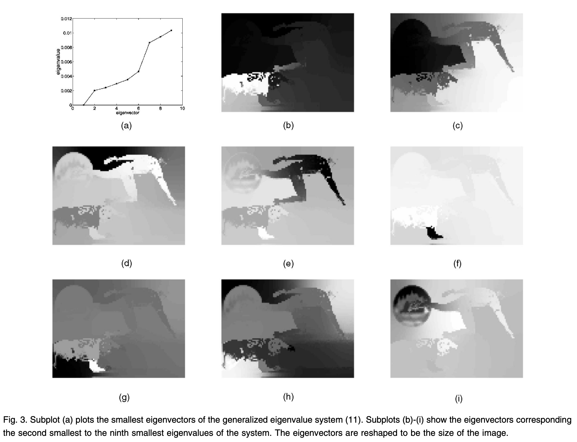
1. Solve the generalized eigensystem for the eigenvectors with the smallest eigenvalues of the system. \(\mathbf{D}^{-\frac{1}{2}}(\mathbf{D} - \mathbf{W})\mathbf{D}^{-\frac{1}{2}}\mathbf{x} = \lambda\mathbf{x}\)

2. Once the eigenvectors are computed, we can partition the graph into two pieces using second smallest eigenvector. but, nonideally our eigenvectors have continuout values and just we need to choose a splitting point to partition it into two parts. normally we can take 0 as splitting point.
3. After the graph is broken into two pieces. we can recursively run our algorithm on the two partitioned parts. Or, we coule take adventage of the other small eigenvectors to partition more than two pieces. but the greater eigenvalue, the lower stability on the partition boundary. as we see in the eigenvector with the seventh to ninth smallest eigenvalues on the bottom picture, the eigenvectors take on the shape of a continuous function rather than discrete that we seek. so we simply choose to ignore all those eigenvetors which have smoothly varying eigenvector values by measuring the degree of smoothness in the eigenvector values and thresholding.

Review

• 이 논문은 분명 기존의 Graph Cut 함수의 문제점과 좋은 Normalized Cut 알고리즘을 제시하고, 계산방법을 제시하였다.
• 특히 제시한 Normalized Cut으로부터 Rayleigh quotient 형식을 이끌어 냈다는 점에서 훌륭한 논문이라고 할 수 있다.
• 하지만 minimized 시키는 방법에 대해서는 의문이 있다. Rayleigh quotient의 solution을 구하는 식 \(\mathbf{D}^{-\frac{1}{2}}(\mathbf{D} - \mathbf{W})\mathbf{D}^{-\frac{1}{2}}\mathbf{x} = \lambda\mathbf{x}\) 은 minimized를 구하는 식이 아닌 critical point를 구하는 식이다. 즉, object function의 값의 법위는 eigenvalue의 값의 범위와 같다. 그렇기에 smallest eigenvalue가 아닌 second smallest eigenvalue는 이 함수의 최소값이라고 단정할 수 없다고 생각한다. 즉 제한 조건이 있는 상태에서 풀어낸 solution의 신뢰성에 의심을 한다. 다만 응용에서 벡터는 이미지 픽셀 전체를 나타내기에 상당히 큰 차원의 벡터를 추정한다. 그렇기에 second smallest eigenvalue은 최솟값일지는 모르겠지만 충분히 작은 값을 나타낸다고 할 수 있고, second가 아닌 그 뒤에 있는 third~ninth까지도 충분히 작은 값을 나타낸다고 볼 수 있다. 또한 모든 eigenvector가 orthogonal 하기 때문에 각각의 eigenvector는 겹치지 않는 고유의 특징을 표현한다고 기대할 수 있겠다.